Spectral filters and frequency analysis

The following functions retrieve frequency spectra from a data series, or apply spectral filters. They are based on signal processing theory and generate faster and more accurate trading signals than traditional indicators. Most filters below are inspired from concepts and ideas by John Ehlers (see book list).

AGC(vars Data, int TimePeriod): var

AGC(vars Data, var alpha): var

Automatic gain control of the Data series, by John Ehlers. Transforms the Data series to the -1 .. +1 range with a fast-attack, slow-decay algorithm. TimePeriod determines the time for reducing the gain by 1.5 db; alternatively, alpha determines the reduction factor per bar period (< 1). Adjustment to higher values happens immediately. The minimum length of the Data series is 1; a single var can be passed with the & operator, f.i. AGC(&MyVariable,10). The function internally creates series (see remarks). Source available in indicators.c. See also scale.

Amplitude(vars Data, int TimePeriod): var

Returns the amplitude - the highest high minus the lowest low - of the Data series, smoothed over the TimePeriod with an EMA so that the more recent fluctuations become more weight.

BandPass(vars Data, int TimePeriod, var Delta): var

Bandpass filter; lets only pass the cycles close to the given TimePeriod. The Delta value (0.05 .. 1) determines the filter width; at Delta = 0.1, cycles outside a 30% range centered at TimePeriod are attenuated with > 3 db. A bandpass filter is useful for retrieving a certain cycle from the data, while ignoring trend and cycles with different periods. The filter can be made steeper by connecting two or more bandpass filters, f.i. BandPass (series (BandPass (Data, TimePeriod, Delta)), TimePeriod, Delta). The minimum length of the Data series is 3. The function internally creates series (see remarks).

Butterworth(vars Data, int CutoffPeriod): var

3-pole Butterworth lowpass filter that suppresses all cycles below the cutoff period. The suppression at the CutoffPeriod is 3 dB. Often used for super-smoothing data. The minimum length of the Data series is 1; a single var can be passed with the & operator, f.i. Butterworth(&MyVariable,10). The function internally creates series (see remarks). Source available in indicators.c.

DominantPeriod(vars Data, int Period): var

Time period of the current dominant cycle in the Data series, in bars; valid range = 10..60 bars, lag = ~10 bars. The dominant cycle is the main periodicity in the data; its period is calculated with a Hilbert transform of the Data series. This function is useful to detect seasonal behavior or to set up moving averages, bandpass or highpass filters so that they adapt to the current market cycle. Period gives the bar period of maximum sensibility. If Data is omitted, the current asset price series is used. The function requires a LookBack period of at least 100 bars. It internally creates series (see remarks).

DominantPhase(vars Data, int Period): var

Current phase angle of the dominant cycle in the Data series, lag corrected; range 0..2*PI. The phase is normally increasing, but can stop or even go backwards when the dominant period is undefined or changes suddenly. The dominant cycle can be synthesized from the data by passing the phase to a sin function (f.i. sin(DominantPhase(Data,30))). This allows determining the maxima and minima of the current market cycle. By adding a constant to the phase (f.i. PI/4), a leading cycle can be generated for detecting the maxima and minima in advance. Period gives the bar period of maximum cycle sensibility. This function also calculates the dominant period; results in rDominantPeriod, rDominantPhase (returned). If Data is omitted, the current asset price series is used. The function requires a LookBack period of at least 100 bars. It internally creates series (see remarks).

FIR3(vars Data): var

FIR4(vars Data): var

FIR6(vars Data): var

Simple finite impulse response lowpass filters with 3, 4, and 6 taps. Often used in more complex filters and indicators for removing noise and smoothing the data. The lag is 1, 1.5, and 2.5 bars; the minimum length of the Data series is equal to the number of taps. Source available in indicators.c

HighPass(vars Data, int CutoffPeriod): var

Wide band highpass filter for separating the cycles in the Data curve from the underlying trend. Attenuates cycles longer than the cutoff period. Often used as an oscillator for identifying price turning points. Compared to traditional oscillators, such as RSI or Stoch, this filter generates much smoother signals with less lag. The minimum length of the Data series is 3, minimum lookback period is 7 bars. The function internally creates series (see remarks).

HighPass1(vars Data, int CutoffPeriod): var

1-pole digital highpass filter, attenuates cycles longer than the cutoff period and returns a curve consisting only of the high frequency part of the data. Often used by other filters for retrieving the cycle part from the data. The minimum length of the Data series is 8. The function internally creates series (see remarks).

HighPass2(vars Data, int CutoffPeriod): var

2-pole digital highpass filte, attenuates cycles longer than the cutoff period and returns a curve consisting only of the high frequency part of the data. The minimum length of the Data series is 3. The function internally creates series (see remarks). Source available in indicators.c.

Laguerre(vars Data, var alpha): var

Laguerre(vars Data, int Period): var

4-element Laguerre lowpass filter. Used for smoothing data similar to an EMA, but with less lag and a wide tuning range given by the smoothing factor alpha (0..1) or alternatively a smoothing period. The low frequency components are delayed much more than the high frequency components, which enables very smooth filters with only a short amount of data. The minimum length of the Data series is 1, the minimum lookback period is 4. The function internally creates series (see remarks). Source available in indicators.c.

LowPass(vars Data, int CutoffPeriod): var

2-pole digital lowpass filter; suppresses high frequencies in the Data series, and thus attenuates all cycles that are shorter than the cutoff period. Compared to an EMA (which is in fact a 1-pole lowpass filter), cycles longer than the cutoff period are unaffected and passed without lag. This allows the LowPass function to react much faster and generate signals earlier than moving averages. Replacing moving averages by lowpass filters improves most algorithms and often makes the difference between a losing and a winning system. The minimum length of the Data series is 3. The function internally creates series (see remarks).

LowPass(var *Buffer, var Value, int CutoffPeriod): var

2-pole digital lowpass filter as above. It does not use series, but keeps its intermediate data in the given Buffer of length 5. The buffer can be an algo-specific array, a static series, or 5 consecutive variables. For instance, LowPass(AssetVar+3,Price,100) uses AssetVar[3]..AssetVar[7] for the buffer. The begin of the buffer is a 3-element series of the LowPass return values and can be used for functions like crossOver, peak, or rising.

Spectrum(vars Data, int TimePeriod, int SamplePeriod): var

Spectral analysis; returns the relative amplitude of the spectral component given by TimePeriod (~5..200). Can be used to analyze the frequency spectrum of a price curve over the given SamplePeriod. The minimum length of the Data series is SamplePeriod; set SamplePeriod (default = 2*TimePeriod) to a multiple of the TimePeriod in order to compensate for spectral dilation. TimePeriod must keep its value from bar to bar, but Spectrum can be called multiple times with different time periods and sample periods during the same bar, for generating a spectrum. The function internally creates series (see remarks). See the Spectrum script and the Strategy chapter for an example.

genNoise(): var

genSine(var Period1, var Period1): var

genSquare(var Period1, var Period2): var

Noise, sine, and square wave chirp generators for testing filters and algorithms. The noise generator produces random noise with 1.0 amplitude. The wave generators generate a hyperbolic chirp with 1.0 amplitude and a wave period changing linearly from Period1 to Period2. For a constant wave period, set both periods to the same value. Source available in indicators.c. See Filter script and example below.

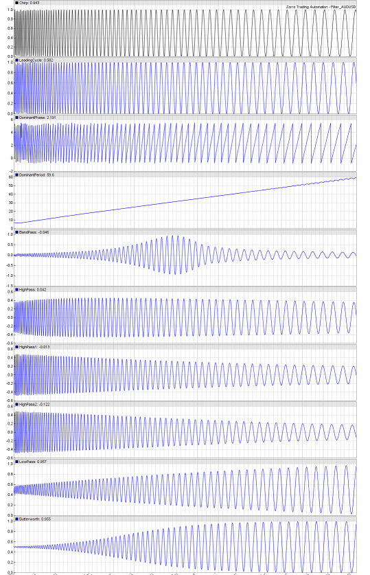
Output of some spectral filters applied to a sine chirp with a period from 5..60 bars (generated by the Filter test script); top to bottom: Data, Leading Cycle, DominantPhase, DominantPeriod, BandPass, HighPass, HighPass1, HighPass2, LowPass, Butterworth.

Standard parameters:

TimePeriod	Number of bars for the time period of the function.
CutoffPeriod	Number of bars for the period that determines the filter frequency.
Data	A data series, often directly derived from the price functions price(), priceClose() etc.. Alternatively a user created series or any other double float array with the given minimum length can be used. If not mentioned otherwise, the minimum length of the Data series is TimePeriod.

Returns:

Filtered value from the Data series.

Remarks:

Most filter functions are available in source code in the script file Source\indicators.c, and can be studied for learning how to code advanced filters and indicators.
Some functions internally create data series, and thus must be called the same number of times and in the same order at any bar. They must therefore not depend on if conditions.
Filter functions are normally cumulative and require a long-enough LookBack period before the filter data is stable. As a rule of thumb, allow about 200 bars lookback period for detecting dominant cycle/phase, 500 bars for highpass and lowpass filters, 1000 bars for bandpass filters, and 2000 bars for spectrum.
All filters can be tested with the Filter script (see above image).

Examples:

// plot some filters  
function run()
{
  set(PLOTNOW);
  vars Price = series(price());

  plot("LowPass",LowPass(Price,20),0,BLUE);
  plot("HighPass",HighPass(Price,50),NEW,RED);
}

// test the dominant cycle detection with a sine chirp
function run()
{
  set(PLOTNOW);
  MaxBars = 2000;
  ColorUp = ColorDn = 0; // don't plot a price curve
  asset(""); // dummy asset
  
  vars Sine = series(genSine(5,60));
  plot("Sine",Sine[0],0,BLACK);
  plot("Period",DominantPeriod(Sine,50),NEW,BLUE);
}

// plot the frequency spectrum of a price curve
function run()
{
  set(PLOTNOW);
  BarPeriod = 60;
  StartDate = 20130101;
  EndDate = 20130201;
  LookBack = 300; // 2 x maximum Cycle

  vars Price = series(price());
  int Cycle;
  for(Cycle = 5; Cycle < 150; Cycle += 1)
    plotBar("Spectrum",Cycle,Cycle,Spectrum(Price,Cycle),BARS+AVG+LBL2,RED);
}