Machine learning algorithms can be used for market prediction with Zorro's advise functions. Due to the low signal-to-noise ratio and to ever-changing market conditions of price series, analyzing the market is an ambitious task for machine learning. But since the price curves are not completely random, even relatively simple machine learning methods, such as in the DeepLearn script, can predict the next price movement with a better than 50% success rate. If the success rate is high enough to overcome transactions costs - at or above 55% accuracy - we can expect a steadily rising profit curve.
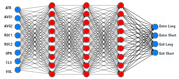
Compared with other machine learning algorithms, such as Random Forests or Support Vector Machines, deep learning systems combine a high success rate with litle programming effort. A linear neural network with 8 analog inputs and 4 binary outputs had a structure like this:
A neural network for trading has normally multiple inputs for price, volume, order book data, indicators etc. and a single analog output that predicts a future price or momentum. Deep learning uses linear or special neural network structures (convolution layers, LSTM) with a large number of neurons and hidden layers. Some parameters common for most neural networks:
Here's a short description of installation and usage of 5 popular R or Python based deep learning packages: Deepnet, Torch, Keras/Tensorflow, H2O, and MxNet. Each comes with an short example of a (not really deep) linear neural net with one hidden layer.
library('deepnet')

neural.train = function(model,XY)
{
  XY <- as.matrix(XY)
  X <- XY[,-ncol(XY)]
  Y <- XY[,ncol(XY)]
  Y <- ifelse(Y > 0,1,0)
  Models[[model]] <<- sae.dnn.train(X,Y,
  hidden = c(30),
  learningrate = 0.5,
  momentum = 0.5,
  learningrate_scale = 1.0,
  output = "sigm",
  sae_output = "linear",
  numepochs = 100,
  batchsize = 100)
}

neural.predict = function(model,X)
{
  if(is.vector(X)) X <- t(X)
  return(nn.predict(Models[[model]],X))
}

neural.save = function(name)
{
  save(Models,file=name)
}

neural.init = function()
{
  set.seed(365)
  Models <<- vector("list")
}
For your convenience, we've uploaded an image of a 64-bit Python installation with Torch and all required modules to https://opserver.de/down/Python312.zip. Unzip it into some folder with full access, like your Documents folder, then enter its path under PythonPath64 in ZorroFix.ini. You need not run a setup or modify the enviroment. Other Python installations on your PC are not affected.
For using Torch, write a .cpp script and run it with the 64-bit Zorro version. Include pynet.cpp, which contains the neural function for Python. Then write the correcponding PyTorch script, with the same name as your strategy, but extension .py. Example:
import torch
from torch import nn
import math
import numpy as np

Path = "Data"
Device = "cpu"
NumSignals = 8
Batch = 15
Split = 90
Epochs = 30
Neurons = 256
Rate = 0.001
Models = []

def neural_init():
    global Device
    Device = (
        "cuda"
        if torch.cuda.is_available()
        else "mps"
        if torch.backends.mps.is_available()
        else "cpu"
    )

def network():
    model = nn.Sequential(
        nn.Linear(NumSignals,Neurons),
        nn.ReLU(),
        nn.Linear(Neurons,Neurons),
        nn.ReLU(),
        nn.Linear(Neurons,1),
        nn.Sigmoid()
    ).to(Device)
    loss = nn.BCELoss()
    optimizer = torch.optim.Adam(model.parameters(),lr=Rate)
    return model,loss,optimizer

def data(Path):
    global NumSignals
    Xy = np.loadtxt(Path,delimiter=',')
    NumSignals = len(Xy[0,:])-1
    return Xy

def split(Xy):
    X = torch.tensor(Xy[:,0:NumSignals],dtype=torch.float32,device=Device)
    y = torch.tensor(Xy[:,NumSignals].reshape(-1,1),dtype=torch.float32,device=Device)
    y = torch.where(y > 0.,1.,0.)
    return X,y

def train(N,Xy):
    global Models
    model,loss,optimizer = network()
    X,y = split(Xy)
    for j in range(Epochs):
        for i in range(0,len(X),Batch):
            y_pred = model(X[i:i+Batch])
            Loss = loss(y_pred,y[i:i+Batch])
            optimizer.zero_grad()
            Loss.backward()
            optimizer.step()
        print(f"Epoch {j}, Loss {Loss.item():>5f}")
    Models.append(model)
    return Loss.item()*100

def neural_train(N,Path):
    Xy = data(Path)
    return train(N,Xy)

def neural_predict(N,X):
    if N >= len(Models):
        print(f"Error: Predict {N} >= {len(Models)}")
        return 0
    model = Models[N]
    X = torch.tensor(X,dtype=torch.float32,device=Device)
    with torch.no_grad():
        y_pred = model(X)
    return y_pred

def neural_save(Path):
    global Models
    torch.save(Models,Path)
    print(f"{len(Models)} models saved")
    Models.clear()

def neural_load(Path):
    global Models
    Models.clear()
    Models = torch.load(Path)
    for i in range(len(Models)):
        Models[i].eval()
    print(f"{len(Models)} models loaded")
Installing the GPU version is more complex, since Tensorflow supports Windows only in CPU mode. So you need to either run Zorro on Linux, or run Keras and Tensorflow under WSL for GPU-based training. Multiple cores are only available on a CPU, not on a GPU.
Example to use Keras in your strategy:
library('keras')

neural.train = function(model,XY)
{
  X <- data.matrix(XY[,-ncol(XY)])
  Y <- XY[,ncol(XY)]
  Y <- ifelse(Y > 0,1,0)
  Model <- keras_model_sequential()
  Model %>%
    layer_dense(units=30,activation='relu',input_shape = c(ncol(X))) %>%
    layer_dropout(rate = 0.2) %>%
    layer_dense(units = 1, activation = 'sigmoid')

  Model %>% compile(
    loss = 'binary_crossentropy',
    optimizer = optimizer_rmsprop(),
    metrics = c('accuracy'))

  Model %>% fit(X, Y,
    epochs = 20, batch_size = 20,
    validation_split = 0, shuffle = FALSE)

  Models[[model]] <<- Model
}

neural.predict = function(model,X)
{
  if(is.vector(X)) X <- t(X)
  X <- as.matrix(X)
  Y <- Models[[model]] %>% predict_proba(X)
  return(ifelse(Y > 0.5,1,0))
}

neural.save = function(name)
{
  for(i in c(1:length(Models)))
    Models[[i]] <<- serialize_model(Models[[i]])
  save(Models,file=name)
}

neural.load = function(name)
{
  load(name,.GlobalEnv)
  for(i in c(1:length(Models)))
    Models[[i]] <<- unserialize_model(Models[[i]])
}

neural.init = function()
{
  set.seed(365)
  Models <<- vector("list")
}
cran <- getOption("repos")
cran["dmlc"] <- "https://s3-us-west-2.amazonaws.com/apache-mxnet/R/CRAN/"
options(repos = cran)
install.packages('mxnet')
The MxNet R script:library('mxnet')
neural.train = function(model,XY)
{
X <- data.matrix(XY[,-ncol(XY)])
Y <- XY[,ncol(XY)]
Y <- ifelse(Y > 0,1,0)
Models[[model]] <<- mx.mlp(X,Y,
hidden_node = c(30),
out_node = 2,
activation = "sigmoid",
out_activation = "softmax",
num.round = 20,
array.batch.size = 20,
learning.rate = 0.05,
momentum = 0.9,
eval.metric = mx.metric.accuracy)
}
neural.predict = function(model,X)
{
if(is.vector(X)) X <- t(X)
X <- data.matrix(X)
Y <- predict(Models[[model]],X)
return(ifelse(Y[1,] > Y[2,],0,1))
}
neural.save = function(name)
{
save(Models,file=name)
}
neural.init = function()
{
mx.set.seed(365)
Models <<- vector("list")
}